Field strength meter for the 137 kHz band by Dick Rollema.

Introduction
The power radiated by an antenna is equal to the radiation resistance multiplied by the antenna current squared. Measurement of antenna current can be done in the 137 kHz band by for instance a thermocouple ammeter or other means. The unknown factor is the radiation resistance. Computer programmes for antenna simulation can produce a value for the radiation resistance but proper modelling the antenna is not always easy. Another problem is the influence of the earth. The ground constants are seldom known and even if they are it is not certain that the computer program applies them in the correct way.
A more reliable way of determining radiated power in the 137 kHz band is by measuring the field strength near the station but outside the near field region. A distance of 1 km is probably sufficient to reduce the influence of the near field on the measurement sufficiently and 2 km is definitely safe.
At such a distance we are in the far field of the antenna but near enough so that the field strength does not depend on the type of ground. When a strength of the electric field of E mV/M is measured the radiated power follows from a simple equation:
P = 0.0111(E *d)2 in which
P in watt
E in mV/m
d in kilometre
* means multiplication
The equation produces the power really radiated by the antenna, in other words the power "dissipated" in the radiation resistance.
Note that this is not the same as ERP. By definition ERP is the fictitious power to be fed to a half wave dipole in free space that produces the measured field strength. As Rik, ON7YD, has pointed out in his e-mail of June 25 a short vertical (and our 137 kHz antennas are always short) has a theoretical gain of a factor 1.83 (2.62 dB) over a half wave dipole in free space. So if you want to know your ERP multiply the power given by equation (1) by 1.83 (or add 2.62 dB). But apart from a regulations point of view I see no advantage in using ERP. The actual power radiated by the antenna is what counts.
I have a feeling that some amateurs talk about their "ERP" when they mean "radiated power". Maybe I'm wrong; I hope so.
Most field strength meters do not measure the electric but the magnetic component of the electromagnetic field. But this is no problem because in the far field of the antenna (where we measure) there is a fixed relation between the electric and the magnetic field components:
E/H=120*pi ohm=377 ohm (2) in which:
E in V/m and H in A/m.
The portable field strength meter to be described is a direct conversion receiver with two audio output signals. One is fed to headphones for tuning the meter to the signal to be measured. The other output feeds a digital multimeter. The voltage indicated by the DVM has a linear relation to the field strength. The meter is calibrated so that a field strength of 5 mV/m produces a reading of 1 V on the DVM.
The instrument can be tuned over the range 135.530 to 139.296 kHz. This includes DCF39 on 138.82 kHz which is useful for comparison purposes.
Description of the instrument
Click here for the full circuit
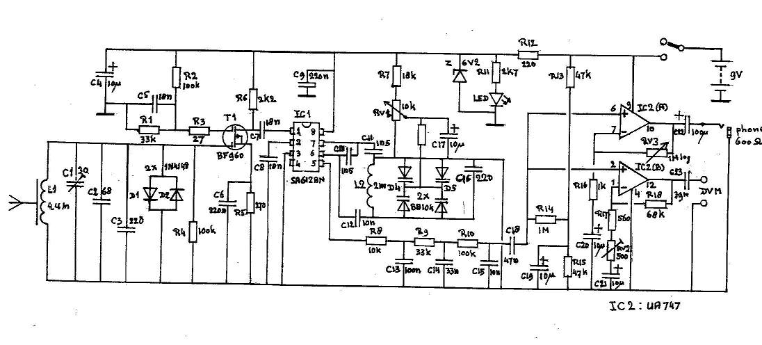

The antenna is a ferrite rod from a broadcast receiver with the original long wave coil in place. The rod is centred in an aluminium tube of 32 mm internal diameter and 145 mm length. I made a slot in the tube to prevent it becoming a short circuited turn. One of the photographs show how the rod is kept in place by two discs of perspex that are glued to the rod.

The electronic circuitry is inside a diecast aluminium box of 120 x 95 x 61 mm. The antenna is tuned by capacitors C1, C2 and C3. C2 and C3 were selected so that C1 can tune the antenna to the centre of the band. It then happened to be at its minimum capacitance as one of the photographs shows. R4 was added to widen the frequency response so that it is sufficiently flat over the range of interest. D1 and D2 protect the meter when used near a live transmitter. T1 amplifies the signal without loading the antenna circuit. It is important in a direct conversion receiver that the signal from the local oscillator cannot reach the antenna circuit. The rf amplifier, including C7, is therefore mounted on a separate piece of copper clad circuit board (not etched, I never use PCB's). Where insulated tie points are required I add small pieces of the same material to the board with instant glue.

The remaining part of the circuitry is on a second board. Here we find the mixer, an IC type SA612BN, incorporating the oscillator circuit. The ubiquitous NE612 can be used as well.

The values of C10, C11 and C16 were dictated by the choice of coil L2. I used a 2 mH hf choke from my junkbox, as shown in one of the photographs. C10 and C11 are the usual capacitors found in a Colpitts oscillator. C12 isolates L2 from the DC on pin 6 of the mixer. I found the BB104 type dual varicaps in my junk box. Two in parallel were necessary to obtain the required tuning range. The lower frequency was set by selecting C16. The upper limit was found to be a bit high and this was corrected by adding R7. RV1 is the tuning control. (The unmarked resistor between the wiper of RV1 and the varicaps is 120 kohm.)
Selectivity of a direct conversion receiver is determined by a low pass filter in the audio path. A high degree of selectivity is required here because of the extremely strong station DCF39 at 138.82 kHz, only 1020 Hz above the upper limit of the band. I use a RC-filter with three sections, each having a time constant RC=1 mS. At first resistors and capacitors of the same value were used in the three sections and this is the situation seen in one of the photographs. Later I realised that a better response is obtained when the loading of a section on its preceding one is decreased and this resulted in the values seen in the circuit diagram. The lower limit of the frequency response is set by the time constant RC=(R17 + RV2)*C21 respectively RC=R16*C20. The response of the metering circuit shows a maximum at about 36 Hz and is 3 dB down at 16 and 88 Hz.
The output of the low pass filter is fed to the two sections of a dual opamp type UA747. The upper opamp feeds the headphones. Volume is controlled by RV3 in the feedback path.
The lower opamp feeds a digital multimeter that must be capable of measuring AC in the millivolt range up to about 2 V. Preset resistor RV2 is adjusted when calibrating the instrument. I choose to make the audio output, as indicated by the DVM, 1000 mV when the instrument is placed in a field of 5 mV/m. The reading is linear up to about 10 mV/m maximum (2 V on the meter).
The instrument is fed by a 9 V battery. The LED is a small one that gives a clear indication of the instrument being switched on when drawing a current of only 2 mA.
To make the gain of the RF amplifier and mixer independent of battery voltage the supply for these stages is stabilized at 6.2 V by a zener diode. R12 was selected so that the zener keeps control for battery voltages down to 7 V. There is no need to stabilize the supply for the opamps because their gain is controlled by negative feedback and therefore hardly depending on the supply voltage. The instrument draws about 17 mA from a new battery.
Calibration
To calibrate the field strength meter the instrument must be placed in a magnetic field of known strength. This can be produced by a pair of so called "Helmholtz coils".

German scientist Helmholtz had in the 19th century found by computation that a homogeneous magnetic field can be produced by placing two circular one-turn coils of radius r metres parallel to each other at a distance of r metres and with their axes coaxial. When a current I is made to flow through each of the coils in the same direction a homogeneous field of H=I/(1.40*r) (3) is generated in a considerable volume between the coils. H in A/m; I in amps; r in m.
I constructed a pair of Helmholtz coils with r=0.292 m as shown in one of the photographs. The coils are connected in parallel and in series with a 50 ohm resistor. At 137 kHz the reactance of the coils is so low that it can be neglected against the 50 ohm resistor. Therefore when the coil pair in series with 50 ohm is connected to a signal generator with U volt output the current I through the coils in parallel is I=U/50. (I in amps). Note that each of the coils carries half of that current.
To check my set-up I made a single turn coil of 10 cm diameter and connected it via a coaxial cable to a selective level meter. I had calculated that with 1 volt applied to the Helmholtz coils in series with 50 ohm a voltage of 208 microvolt should be induced in the 10 cm coil when held between the Helmholtz coil pair. I measured 210 microvolt! Almost too good to be true. But upon checking everything again I found nothing wrong.
As I wanted the field strength meter to produce a reading of 1000 mV in a field strength of 5 mV meter I applied equation (2) and found that the corresponding magnetic field component is H=13.3*10-6 A/m. Using equation (3) the generator output voltage was found that would result in the wanted field between the Helmholtz coils. The field strength meter was put between the coils and RV2 adjusted for a voltage of 1000 mV on the digital multimeter. That completed calibration.
Measuring field strength
Try to find an open space at least 1 kilometre from the transmitter. Keep the antenna of the meter horizontal and tune the signal to zero beat. Now slowly increase or decrease the tuning slightly for a maximum reading on the DVM. Whether or not you can hear the beat note of about 36 Hz depends on the quality of your headphones. Turn around slowly to find the position for maximum signal. Now walk around a bit. If the reading varies the field is distorted by for instance a metallic fence, a lamppost or underground cables or pipelines. (On 137 kHz the waves penetrate tens of metres into the earth!) When a constant indication is found, multiply the reading in volt by five to obtain the field strength in mV/m.
Find the distance to the transmitter on a map or by other means (GPS!). Apply equation (1) to find radiated power. Multiply by 1.83 if ERP is required.
Good luck!
73, Dick, PA0SE
Download the article (Word2) and pictures as a zip file (223k)